Newly Blog

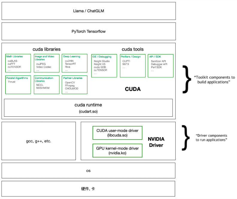
GPU

• look up GPU information: lspci or lshw -C display

• NVIDIA system management interface, monitor GPU usage: nvidia-smi (GPU driver version and CUDA user-mode version)

GPU Driver

• check the latest driver information on http://www.nvidia.com/Download/index.aspx. Then, look up driver information on local machine: cat /proc/driver/nvidia/version

• check the compatibility between CUDA runtime version and driver version: https://docs.nvidia.com/deploy/cuda-compatibility/

• Install NVIDIA GPU driver using GUI: Software & Updates -> Additional Drivers

• Install NVIDIA GPU driver using apt-get

  1 2 3

  sudo add-apt-repository ppa:Ubuntu-x-swat/x-updates sudo apt-get update sudo apt-get install nvidia-current nvidia-current-modaliases nvidia-settings

• Install NVIDIA GPU driver using *.run file downloaded from http://www.nvidia.com/Download/index.aspx

  1. Hit CTRL+ALT+F1 and login using your credentials.
  2. Stop your current X server session by typing sudo service lightdm stop
  3. Enter runlevel 3 by typing sudo init 3 and install your *.run file.
  4. You might be required to reboot when the installation finishes. If not, run sudo service lightdm start or sudo start lightdm to start your X server again.

CUDA

When using anaconda to install deep learning platform, sometimes it is unnecessary to install CUDA by yourself.

1. Preprocessing

   • uninstall the GPU driver first: sudo /usr/bin/nvidia-uninstall or sudo apt-get remove --purge nvidia* and sudo apt-get autoremove; sudo reboot
   • blacklist nouveau: add “blacklist nouveau” and “options nouveau modeset=0” at the end of /etc/modprobe.d/blacklist.conf; sudo update-initramfs -u; sudo reboot
   • Stop your current X server session: sudo service lightdm stop

2. Install Cuda

   Download the *.run file from NVIDIA website

   • The latest version: https://developer.nvidia.com/cuda-downloads

   • All versions: https://developer.nvidia.com/cuda-toolkit-archive

     1	sudo sh cuda_10.0.130_410.48_linux.run

     and then add into PATH and LD_LIBRARY_PATH

     1 2 3

     echo 'export PATH=/usr/local/cuda/bin:$PATH' >> ~/.bashrc echo 'export LD_LIBRARY_PATH=/usr/local/cuda/lib64:$LD_LIBRARY_PATH' >> ~/.bashrc source ~/.bashrc

3. check Cuda version after installation: nvcc -V. Compile and run the cuda samples.

CuDNN

CuDNN is to accelerate Cuda, from https://developer.nvidia.com/rdp/form/cudnn-download-survey, just download compressed package.

1
2
3

cd $CUDNN_PATH	
sudo cp include/* /usr/local/cuda/include/
sudo cp -P lib64/* /usr/local/cuda/lib64/ #use -P to retain symbolic links

1. Dichromatic Reflection Model [1] [2] $I_i=\gamma_b C_i L_i R_{b,i}+\gamma_s C_i L_i R_{s,i}$, in which $i$ is the pixel index, $L$ is the global illumination, $C_i$ is the sensor sensitivity. The chromatic terms $R_b$ and $R_s$ account for body and surface reflection, which are only related to object material.

2. gray pixels: pixels with equal RGB values. detecting gray pixels in a color-biased image is not easy. [3]

3. albedo, shading, gloss [4] [5]

Reference

[1] Shafer, Steven A. “Using color to separate reflection components.” Color Research & Application 10.4 (1985): 210-218.
[2] Song, Shuangbing, et al. “Illumination Harmonization with Gray Mean Scale.” Computer Graphics International Conference. Springer, Cham, 2020.
[3] Qian, Yanlin, et al. “On finding gray pixels.” CVPR, 2019.
[4] Bhattad, Anand, and David A. Forsyth. “Cut-and-Paste Neural Rendering.” arXiv preprint arXiv:2010.05907 (2020).
[5] Yu, Ye, and William AP Smith. “InverseRenderNet: Learning single image inverse rendering.” CVPR, 2019.

Interface Type:

GigE and USB interfaces are commonly used. The advantage of GigE is long-distance transmission.

Color v.s. Monochrome

When the exposure begins, each photosite is uncovered to collect incoming light. When the exposure ends, the occupancy of each photosite is read as an electrical signal, which is then quantified and stored as a numerical value in an image file.

Unlike color sensors, monochrome sensors capture all incoming light at each pixel regardless of color.
Unlike with color, monochrome sensors also do not require demosaicing to create the final image because the values recorded at each photosite effectively just become the values at each pixel. As a result, monochrome sensors are able to achieve a slightly higher resolution.

Sensor Type:

• CCD (Charged Coupling Devices): special manufacturing process that allows the conversion to take place in the chip without distortion, which makes them more expensive. CCD can capture high-quality image with low noise and is sensitive to light.

• CMOS (Complimentary Metal Oxide Semiconductor): use transistors at each pixel to move the charge through traditional wires. Traditional manufacturing processes are used to make CMOS, which is the same as creating microchips. CMOS is cheaper and has low power consumption

Readout Method:

Global v.s. rolling shutter: originally, CCD uses global shutter while CMOS uses rolling shutter. Rolling shutter is always active and rolling through the pixels line by line from top to bottom. In contrast, global shutter stores their electrical charges and reads out when the shutter is closed and the pixel is reset for the next exposure, allowing the entire sensor area to be output simultaneously. Nowadays, CMOS can also have global shutter capabilities.

Advantage of global shutter: global shutter can manage motions and pulsed light conditions rather well as the scene is viewed or exposed at one moment in time by enabling synchronous timing of the light or motion to the open shutter phase. However, rolling shutter can also manage motions and pulsed light conditions to an extent through a combination of fast shutter speeds and timing of the light source.

Quantum Efficiency

The ability of a pixel to convert an incident photon to charge is specified by its quantum efficiency. For example, if for ten incident photons, four photo-electrons are produced, then the quantum efficiency is 40%. Typical values of quantum efficiency are in the range of 30 - 60%. The quantum efficiency depends on wavelength and is not necessarily uniform over the response to light intensity.

Field of View

FOV (Field of View) depends on the lens size. Generally, larger sensors yield greater FOV.

Pixel Size

A small pixel size is desirable because it results in a smaller die size and/or higher spatial resolution; a large pixel size is desirable because it results in higher dynamic range and signal-to-noise ratio.

Multi-agent RL: [1]

Reference

[1] Deng, Zehao, et al. “Training High-Level Schedulers with Execution-Feedback Reinforcement Learning for Long-Horizon GUI Automation.” arXiv preprint arXiv:2511.22235 (2025).

(1) Zoom in a bounding box [1] [2]

(2) Zoom in salient region [3] [4]

• relation to (1): if the salience region is rectangle and salience value is infinity, this should be equivalent to zooming in a bounding box.
• relation to pooling: weighted pooling with salience map as weight map
• relation to deformable CNN: use salience map to calculate offset for each position

Reference

[1] Fu, Jianlong, Heliang Zheng, and Tao Mei. “Look closer to see better: Recurrent attention convolutional neural network for fine-grained image recognition.” CVPR, 2017.

[2] Zheng, Heliang, et al. “Learning multi-attention convolutional neural network for fine-grained image recognition.” ICCV, 2017.

[3] Recasens, Adria, et al. “Learning to zoom: a saliency-based sampling layer for neural networks.” ECCV, 2018.

[4] Zheng, Heliang, et al. “Looking for the Devil in the Details: Learning Trilinear Attention Sampling Network for Fine-grained Image Recognition.” arXiv preprint arXiv:1903.06150 (2019).

Survey

For a brief survey summarizing skip-gram, CBOW, GloVe, etc, please refer to this.

Code

word2vec: TensorFlow

GloVe: C, TensorFlow

WikiCorpus

Download the WikiCorpus and use the shellscript to process (e.g., remove numbers, invalide chars, urls), leading to sequence of pure words.

Resources

• English word vectors: https://github.com/3Top/word2vec-api
• Non-English word vectors: https://github.com/Kyubyong/wordvectors

Problem

Tracking is challenging due to the following factors: deformation, illumination variation, blur&fast motion, background clutter, rotation, scale, boundary effect

History

Tracking methods can be roughly categorized into generative methods and discriminative methods(feature+machine learning). Recently, correlation filter based methods and deep learning methods are dominant.

• Meanshift: density based, ASMS https://github.com/vojirt/asms
• Particle filter: particle based statistical method
• Optical flow: match feature points between neighboring frames
• correlation filter: KCF, DCF, CSK, CN, DSST, SRDCF, ECO. Basic CF methods are sensitive to deformation, fast motion, and boundary effect.
• deep learning: GOTURN, MDNet, TCNN, SiamFC

Two research groups contribute to CF methods most:

• Oxford: https://www.robots.ox.ac.uk/~luca/,
• Linkoping: http://users.isy.liu.se/en/cvl/marda26/

Comparison of Speed and Performance

Survey papers

• Object tracking: A survey, 2006
• Object tracking benchmark, 2015

Benchmark

• OTB50/100: http://cvlab.hanyang.ac.kr/tracker_benchmark/
• VOT2016: http://www.votchallenge.net/vot2016/dataset.html

Challenge

• Visual Object Tracking (VOT) challenge:
  http://www.votchallenge.net/challenges.html
  VOT2016 has released the code of many trackers: http://votchallenge.net/vot2016/trackers.html
• Multiple Object Tracking Challenge (MOT) challenge:
  https://motchallenge.net/

Detection based Tracking

Detection based tracking is also named as tracking by detection or multiple object tracking. (MOT Challenge)

TLD (tracking-learning-detection): update tracker and detector during learning
http://personal.ee.surrey.ac.uk/Personal/Z.Kalal/tld.html

1. Joint Image Emotion Classification and Distribution Learning via Deep Convolutional Neural Network

2. Weakly Supervised Coupled Networks for Visual Sentiment Analysis

Visual dialogue [1]: a dialogue with one image

Multimodal Dialogue [2][3]: a dialogue with multiple images

[1] Visual Dialog

[2] Towards Building Large Scale Multimodal Domain-Aware Conversation Systems

[3] Knowledge-aware Multimodal Dialogue Systems

warping

• correspondence matrix [1] [4]
• TPS [1] [3]
• offset and weight [2]

target person

Garment Transfer: [5] [6] [8]

Controllable person image synthesis: [7]

Recurrent Person Image Generation: [9]

References

1. Yang, Fan, and Guosheng Lin. “CT-Net: Complementary Transfering Network for Garment Transfer with Arbitrary Geometric Changes.” CVPR, 2021.

2. Bai, Shuai, et al. “Single Stage Virtual Try-on via Deformable Attention Flows.” arXiv preprint arXiv:2207.09161 (2022).

3. Fenocchi, Emanuele, et al. “Dual-Branch Collaborative Transformer for Virtual Try-On.” CVPR, 2022.

4. Morelli, Davide, et al. “Dress Code: High-Resolution Multi-Category Virtual Try-On.” CVPR, 2022.

5. Fan Yang, Guosheng Lin. “CT-Net: Complementary Transfering Network for Garment Transfer with Arbitrary Geometric Changes.” CVPR, 2021.

6. Liu, Ting, et al. “Spatial-aware texture transformer for high-fidelity garment transfer.” IEEE Transactions on Image Processing 30 (2021): 7499-7510.

7. Zhou, Xinyue, et al. “Cross Attention Based Style Distribution for Controllable Person Image Synthesis.” arXiv preprint arXiv:2208.00712 (2022).

8. Raj, Amit, et al. “Swapnet: Image based garment transfer.” European Conference on Computer Vision. Springer, Cham, 2018.

9. Cui, Aiyu, Daniel McKee, and Svetlana Lazebnik. “Dressing in order: Recurrent person image generation for pose transfer, virtual try-on and outfit editing.” ICCV, 2021.