Difference between VM and Docker
VM: guest OS -> BINS&LIBS -> App
Docker: BINS*LIBS -> App
Installation
https://docs.docker.com/engine/install/ubuntu/
Uninstallation
- Uninstall the Docker Engine, CLI, containerd, and Docker Compose packages:
sudo apt-get purge docker-ce docker-ce-cli containerd.io docker-buildx-plugin docker-compose-plugin docker-ce-rootless-extras
- Images, containers, volumes, or custom configuration files on your host aren’t automatically removed. To delete all images, containers, and volumes:
sudo rm -rf /var/lib/docker, sudo rm -rf /var/lib/containerd
Commands
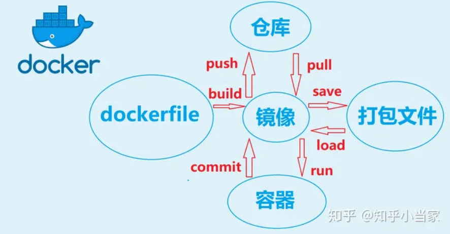
image
docker image pull $image_name:$version
docker image tag $image_name:version $registryIP:port/username/image_name:version
docker image push $registryIP:port/username/image_name:version
docker image build -t $image_name .
docker image ls
docker image rm $image_name
docker image save $image_name > $filename
docker load < $filename
container
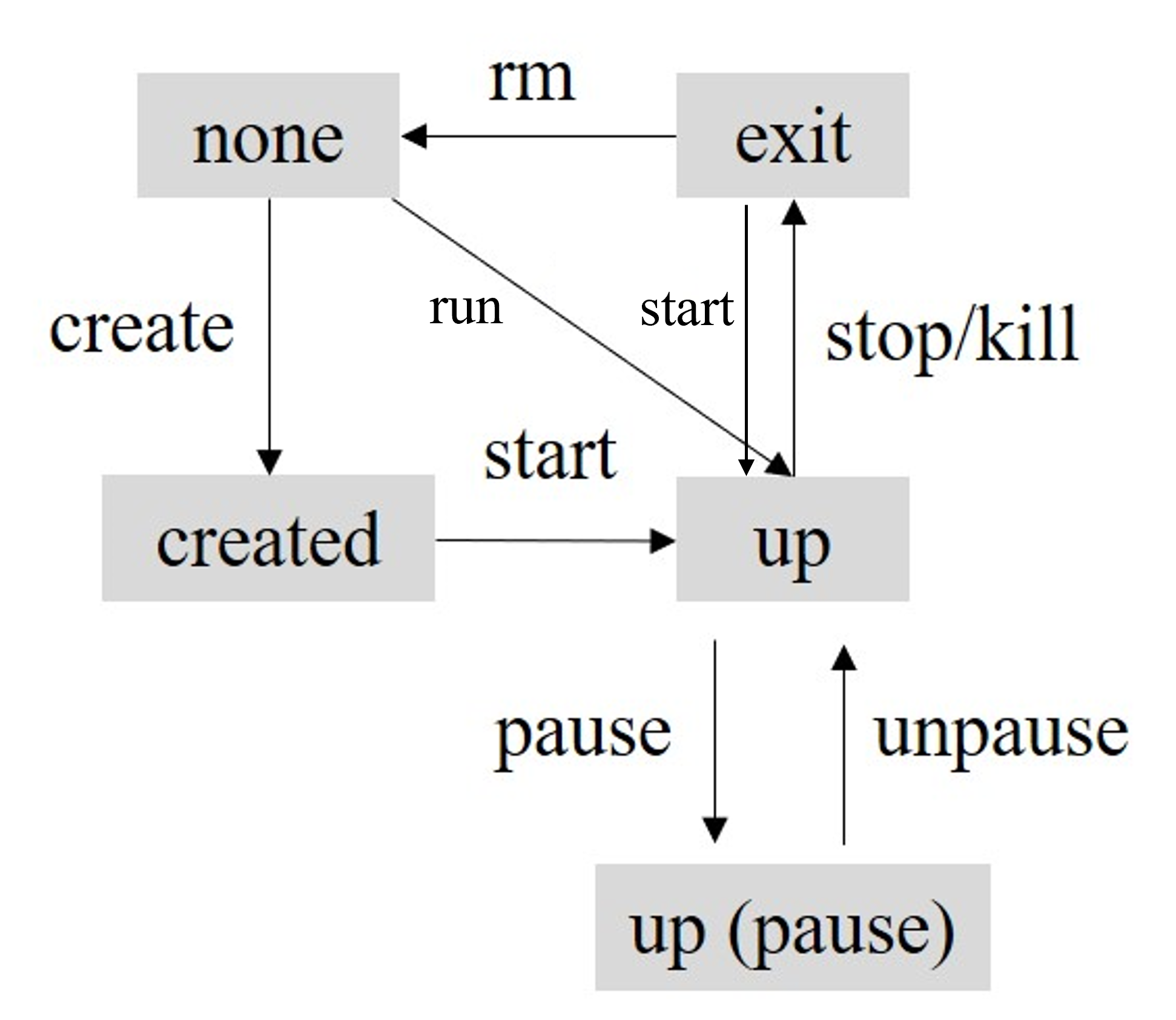
docker container create $image_name
docker container start $container_ID
docker container run $image_name # run is equal to create and start
docker container run -it $image_name /bin/bash
docker container ls, docker container ls --a
docker container pause $container_ID
docker container unpause $container_ID
docker container stop $container_ID
docker container kill $container_ID # the difference between stop and kill is that stop may do some clean-up before killing the container
docker container rm $container_ID
docker container prune # remove all the exit containers
docker container exec -it $containe_ID /bin/bash
docker container cp $container_ID:$file_path .
docker container commit $container_ID $image_name:$version
Dockerfile
FROM python:3.7
WORKDIR ./docker_demo
ADD . .
RUN pip install -r requirements.txt
CMD ["python", "./src/main.py"]
Tutorial: [1]
Use GPU in docker
Install nvidia-docker https://docs.nvidia.com/datacenter/cloud-native/container-toolkit/latest/install-guide.html
docker run --gpus all -it $image_name